Chapter 11Integration and the fundamental theorem of calculus
"One should never try to prove anything that is not almost obvious"
- Alexander Grothendieck
This guy, Grothendieck, is somewhat of a mathematical idol to me. And I just love this quote, don't you? Too often in math we just dive into showing that a certain fact is true with long series of formulas before stepping back and making sure that it feels reasonable, and preferably obvious, at least on an intuitive level.
In this article, I want to talk about integrals, and the thing that I want to become "almost obvious" is that they are an inverse of derivatives. We'll focus just on one example, which is kind of dual to the example of a moving car that I talked about in chapter 2 of the series, introducing derivatives. Then in the next lesson, we'll see how the idea generalizes into some other contexts.
Velocity
Imagine you're sitting in a car, and you can't see out the window; all you see is the speedometer. At some point, the car starts moving, speeds up, then slows back down to a stop, all over 8 seconds.

Is there a nice way to figure out how far you've traveled during that time, based only on your view of the speedometer? Or better yet, find a distance function that tells you how far you've traveled after any given amount of time, , between 0 and 8 seconds. Let's say you take note of the velocity at each second, and make a plot over time like this.

And maybe you find that a nice function to model your velocity over time, in meters per second, is .

Relationship between velocity and distance
You might remember, in chapter 2 of this series, we were looking at the opposite situation, where you know a distance function, , and you want to figure out a velocity function from that. I showed how the derivative of your distance vs. time function gives you a velocity vs. time function.

So in our current situation, where all we know is the velocity function, it should make sense that finding a distance vs. time function comes down to asking what function has a derivative . This is often described as finding the antiderivative of a function.

And indeed, that's what we'll end up doing, and you could even pause and try that right now for the function .

But first, I want to spend the bulk of this article showing how this question is related to finding an area bounded by the velocity graph, because that helps to build an intuition for a whole class of what are called "integral problems" in math and science.

This figure highlights the area bounded under the curve formed by the function . The vertical axis represents velocity measured in meters per second and the horizontal axis reprents time.
To start off, notice this question would be much easier if the car was moving with a constant velocity, right? In that case, you could just multiply the velocity, in meters per second, by the amount of time passed, in seconds, and that gives you the number of meters traveled.

Notice that you can visualize that distance as an area, and if visualizing distance as an area seems weird, I'm right there with you. It's just that on this plot, where the horizontal direction has units of seconds and the vertical direction has units of meters/second, units of area very naturally correspond to meters. But what makes our situation hard is that the velocity is not constant, it's incessantly changing at every instant.
It would even be a lot easier if it only ever changed at a handful of points, maybe staying static for the first second, then suddenly discontinuously jumping to a constant 7 meters per second for the next second, and so on, with discontinuous jumps to portions of constant velocity.

That might make it very uncomfortable for the driver, in fact, it's physically impossible, but it would make your calculations a lot more straightforward. You could compute the distance traveled on each interval by multiplying the constant velocity on that interval by the change in time. Then just add them all up.

So what we'll do is just approximate our velocity function as if it was constant on a bunch of different intervals. Then, as is common in calculus, we'll see how refining that approximation leads us to something precise.

Notice as the we choose more and more sub-divisions that these approximations start to approach the true shape of the area bounded by the curve.
Here, let's make this more concrete with some numbers. Chop up the time axis between 0 and 8 into many small intervals, each with some little width , like 0.25 seconds. Consider one of these intervals, like the one between , and . In reality, the car speeds up from 7 m/s to about 8.4 m/s during that time, which you can find by plugging in and 1.25 to the equation for velocity.

We want to approximate the car's motion as if its velocity was constant on this interval. Again, the reason for doing that is that we don't really know how to handle anything other than constant velocity situations. You could choose this constant to be anything between and , it doesn't really matter.
All that matters is that our sequence of approximations, whatever they are, gets better and better as gets smaller and smaller. Treating this car's journey as a bunch of discontinuous jumps in speed between small portions of constant velocity becomes a less wrong reflection of reality as we decrease the time between those jumps.
So, for convenience, let's just approximate the speed on each interval with whatever the true car's velocity is at the start of the interval; the height of the graph above the left side, which in this case is 7.

So on this example interval, according to our approximation, the car moves . That's meters, nicely visualized as the area of this thin rectangle. This is a little under the real distance traveled, but not by much. And the same goes for every other interval: The approximated distance is , it's just that you plug in a different value of for each one, giving a different height for each rectangle.
Integral Notation
I'm going to write out an expression for the sum of the areas of all these rectangles in kind of a funny way. Take this symbol , which looks like a stretched "S" for sum, then put a at its bottom and an at its top to indicate that we're ranging over time steps between and seconds.

The amount we're adding up at each time step is which, for each step, can be visualized as the rectangle of area on the graph.

Two things are implicit in this notation: First, the value plays two roles: not only is it a factor in each quantity we're adding up, it also indicates the spacing between each sampled time step. So when you make smaller, even though it decreases the area of each rectangle, it increases the total number of rectangles whose areas we're adding up, because if they are thinner it takes more of them to fill up that space. And second, the reason we don't use the usual sigma notation to indicate a sum is that this expression is technically not any particular sum for any particular choice of ; it's meant to express whatever that sum approaches as approaches 0.

As approaches the area of the rectangle approaches the area bounded by the curve and the horizontal axis.
Remember, smaller choices of indicate closer approximations for our original question, how far does the car go? So this limiting value for the sum, the area under this curve, gives the precise answer to the question, in full unapproximated precision.

Area under the curve is equal to the distance traveled.
Now tell me that's not surprising. We have this pretty complicated idea of approximations that can involve adding up a huge number of very tiny things, and yet the value those approximations approach can be described so simply, as the area under a curve.
This expression is called an "integral" of , since it brings all of its values together, it integrates them.
Area Under Graphs
Now you could say, "How does this help!? You've just reframed one hard question, finding how far the car has traveled, into another equally hard problem, finding the area between this graph and the horizontal axis?" And...you'd be right! If the velocity/distance duo was all we cared about, most of this video with all this area under a curve nonsense would be a waste of time. We could just skip straight ahead to figuring out an antiderivative.
But finding the area between a function's graph and the horizontal axis is somewhat of a common language for many disparate problems that can be broken down and approximated as the sum of a large number of small things. You'll see more next lesson, but for now I'll just say in the abstract that understanding how to interpret and compute the area under a graph is a very general problem-solving tool.
In fact, the first video of this series already covered the basics of how this works, but now that we have more of a background with derivatives, we can actually take the idea to its completion.
Derivative of area function is the function
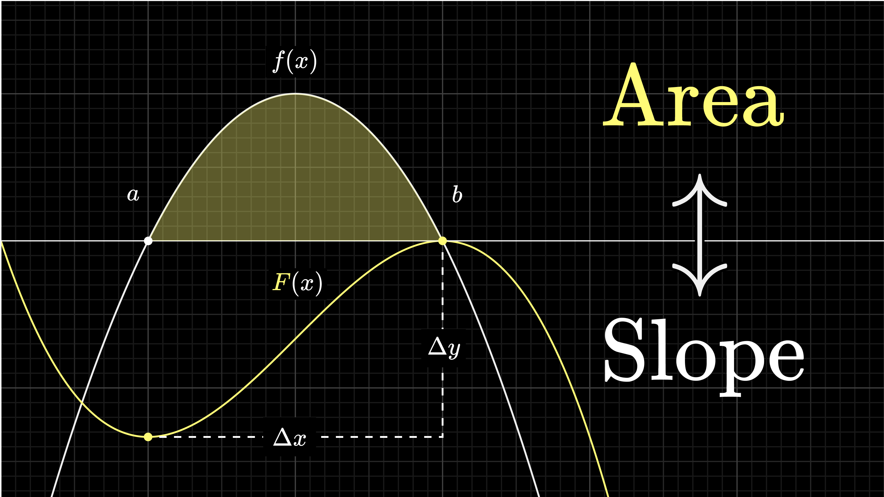
For our velocity example, think of this right endpoint as a variable, capital .

So we're thinking of this integral of the velocity function between and , the area under this curve between those two inputs, as a function, where that upper bound is the variable. That area represents the distance the car has traveled after seconds, right? So this is really a distance vs. time function .

Now ask yourself: What is the derivative of that function? On the one hand, a tiny change in distance over a tiny change in time is velocity; that's what velocity means. But there's another way to see it purely in terms of this graph and this area, which generalizes better to other integral problems.

A slight nudge of to the input causes that area to increase, some little represented by the area of this sliver. The height of that sliver is the height of the graph at that point, , and its width is . And for small enough , we can basically consider that sliver to be a rectangle. So the area of that sliver, , is approximately equal to .
Because this approximation gets better and better for smaller , the derivative of the area function at this point equals , the value of the velocity function at whatever time we started on.

And that's super general, the derivative of any function giving the area under a graph like this is equal to the function for the graph itself.

Find the antiderivative
So if our velocity function here is , what should be? What function of has a derivative ? This is where we actually have to roll up our sleeves and do some math.

It's easier to see if we expand this out as . Take each part here one at a time: What function has a derivative ? Well, we know that the derivative of is , so if we just scale that up by , we see that the derivative of is .
And for that second part, what kind of function might have as its derivative? Using the power rule again, we know that the derivative of a cubic term, , gives a squared term, , so if we scale that down by a third, the derivative of is exactly , and making that negative we see that has a derivative of .
Therefore, the antiderivative of our function is .
What is the antiderivative of the function ?
What is the antiderivative of the function ?
The +C issue
But there's a slight issue here: we could add any constant to this function, and its derivative would still be . The derivative of a constant is always 0. And if we graph , you can think of this in the sense that moving a graph of a distance function up and down does nothing to affect its slope above each input. So there are actually infinitely many different possible antiderivative functions, all of which look like for some constant .

But there is one piece of information we haven't used yet that lets us zero in on which antiderivative to use: The lower bound on the integral. This integral must be zero when we drag that right endpoint all the way to the left endpoint, right?

The distance traveled by the car between 0 seconds and 0 seconds is zero. So as we found, this area as a function of capital is an antiderivative for the stuff inside, and to choose what constant to add, subtract off the value of that antiderivative function at the lower bound. If you think about it for a moment, that ensures that the integral from the lower bound to itself will indeed be 0.
As it so happens, when you evaluate the function we have here at , you get zero, so in this specific case you don't actually need to subtract off anything. For example, the total distance traveled during the 8 seconds is this expression evaluated at , which is , minus 0 which is the answer to our original question! But a more typical example would be something like this integral between and . That's the area pictured here, and it represents the distance traveled between 1 second and 7 seconds.

What you'd do is evaluate the antiderivative we found at the top bound, , and subtract off its value at the bottom bound, . Notice, it doesn't matter what antiderivative we choose here; if for some reason it had a constant added to it, like , that constant would cancel out.
What is the distance traveled by a car between and seconds whose velocity is modeled by the function ? This car starts at a speed of 20 meters per second and slows down at a constant rate.
What is the distance traveled by a car between and seconds whose velocity is modeled by the function ?
Fundamental theorem

More generally, anytime you want to integrate some function - and remember you think of as adding up the values for inputs in a certain range then asking what that sum approaches as approaches - the first step to evaluating that integral is to find an antiderivative, some other function, "capital ", whose derivative is the thing inside the integral. Then the integral equals this antiderivative evaluated at the top bound, minus its value at the bottom bound. This fact is called the "fundamental theorem of calculus".

Here's what's crazy about this fact: The integral, the limiting value for the sum of all these thin rectangles, takes into account every single input on the continuum from the lower bound to the upper bound, that's why we use the word "integrate"; it brings them together. And yet, to actually compute it using the antiderivative, you look at only two inputs: the top bound and the bottom bound. It almost feels like cheating! Finding the antiderivative implicitly accounts for all the information needed to add up all the values between the lower bound and upper bound.
Quick recap
There's kind of a lot packed into this whole concept, so let's recap everything that just happened. We wanted to figure out how far a car goes just by looking at the speedometer, and what makes that hard is that the velocity was always changing.

If you approximate it to be constant on multiple different intervals, you can figure out how far the car goes on each interval just with multiplication, then add them all up. Adding up those products can be visualized as the sum of the areas of many thin rectangles like this.

Better and better approximations of the original problem correspond to collections of rectangles whose aggregate area is closer and closer to being the area under this curve between the start time and end time, so that area under the curve is the precise distance traveled for the true, nowhere-constant velocity function.

As dt approaches 0 the aggregate area is closer and closer to being the area under this curve which is the precise distance traveled between the start and end time
If you think of this area as function, with a variable right end point, you can deduce that the derivative of that area function must equal the height of the graph at each point.

That's the key! So to find a function giving this area, you ask what function has as its derivative.
There are actually infinitely many antiderivatives of a given function, since you can always just add some constant without affecting the derivative, so you account for that by subtracting off the value of whatever antiderivative function you choose at the bottom bound.
Negative area
By the way, one important thing to bring up before leaving is the idea of negative area. What if our velocity function was negative at some point? Meaning the car is going backwards. It's still true that the tiny distance traveled on a little time interval is about equal to the velocity times the tiny change in time, it's just that the number you'd plug in for velocity would be negative, so that tiny change in distance is negative.
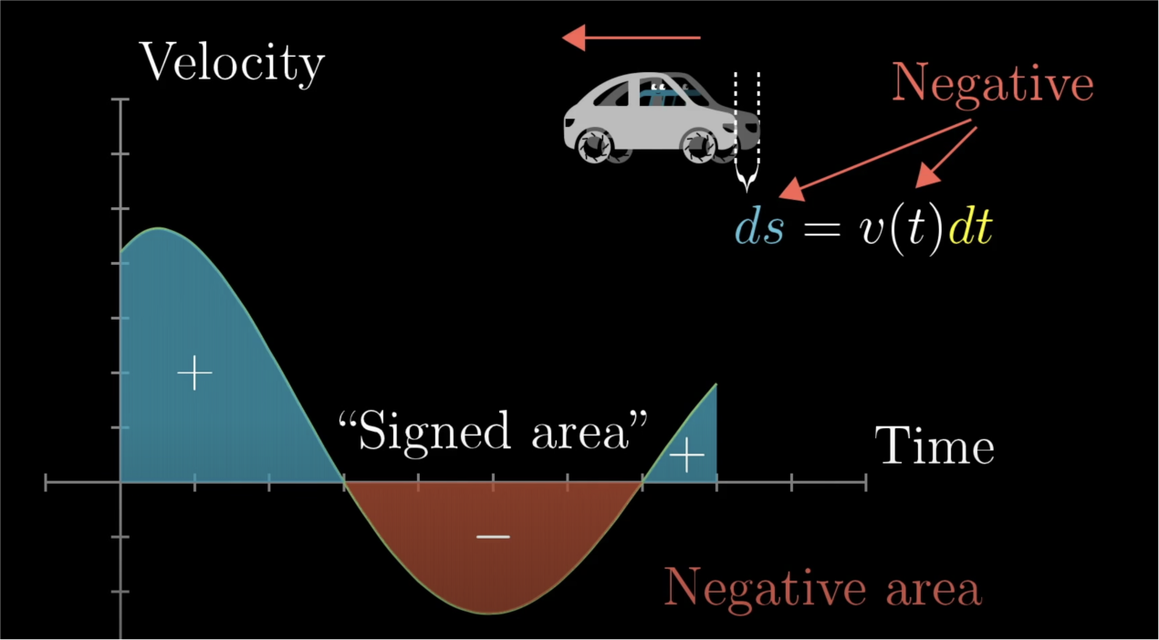
In terms of our thin rectangles, if the rectangle goes below the horizontal axis like this, its area represents a bit of distance traveled backwards, so if what you want is to find the distance between the car's start point and end point, you'd want to subtract it. And this is generally true of integrals: Whenever a graph dips below the horizontal axis, that area underneath is counted as negative. What you'll commonly hear is that integrals measure the "signed" area between a graph and the horizontal axis.
A car starts driving backwards, slows down then starts driving forward with a velocity modeled by the function . At what point in time has the car reached the position it started from?
Next video
Next up I'll bring up more contexts where this idea of an integral and the area under curves comes up, along with some other intuitions for the fundamental theorem of calculus.
Thanks
Special thanks to those below for supporting the original video behind this post, and to current patrons for funding ongoing projects. If you find these lessons valuable, consider joining.