Chapter 4What is backpropagation really doing?
Here we tackle backpropagation, the core algorithm behind how neural networks learn. If you followed the last two lessons or if you’re jumping in with the appropriate background, you know what a neural network is and how it feeds forward information.
Quick Recap
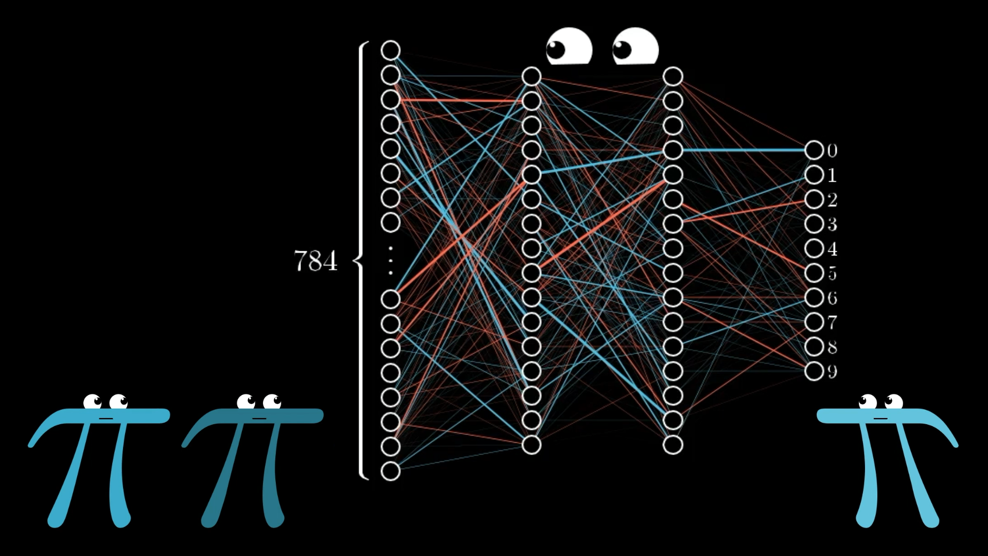
We’ve been looking at the classic example of recognizing handwritten digits. I’ve been showing a network with...
- An input layer of 784 neurons (which represent the pixel values of the image)
- Two hidden layers with 16 neurons each
- An output layer with 10 neurons (indicating the network’s choice of digit)
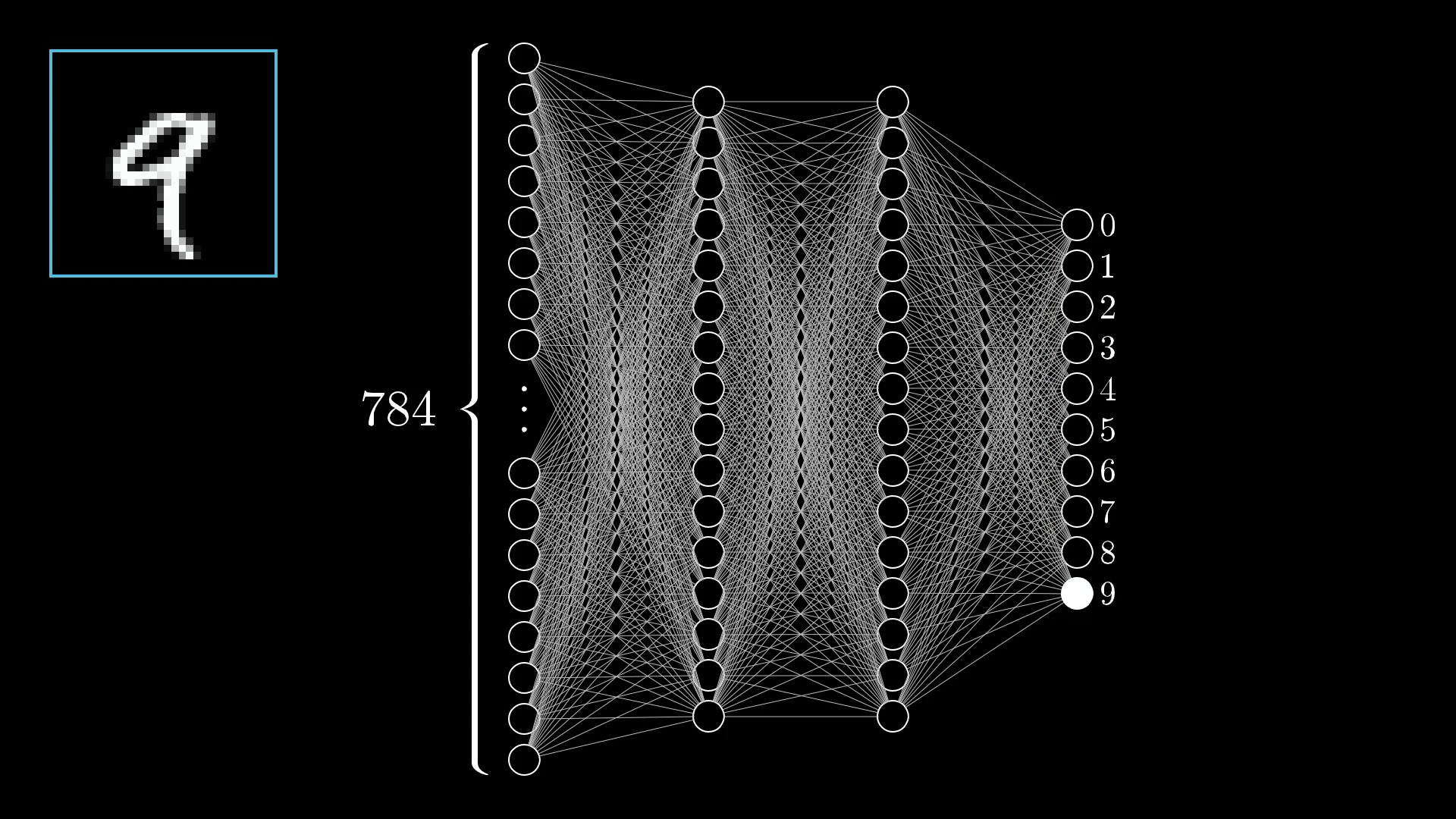
Our basic neural network has four layers: An input layer, an output layer, and two hidden layers in between.
We’ve also discussed gradient descent, so you should know that when people describe a network as “learning,” they mean finding the weights and biases that minimize a certain cost function.
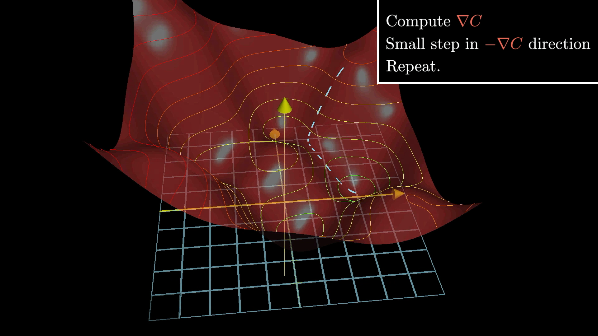
We use gradient descent to walk downhill to a local minimum of the cost function.
To calculate the cost of a single training example, you take the output that the network gives, along with the output you wanted it to give, and you add up the squares of the differences between each component:
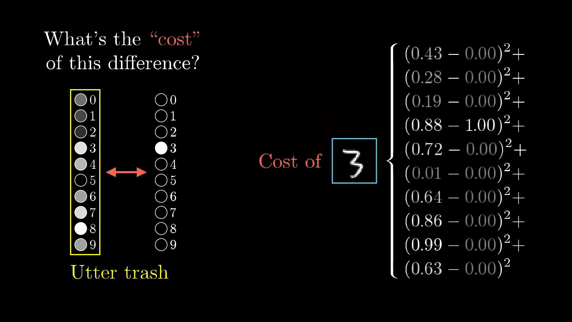
The cost for a single training example is the sum of the squares of the differences between the actual output and the desired output.
Doing this for all your tens of thousands of training examples, and averaging all the results, gives you the total cost of the network.
What is Backpropagation?
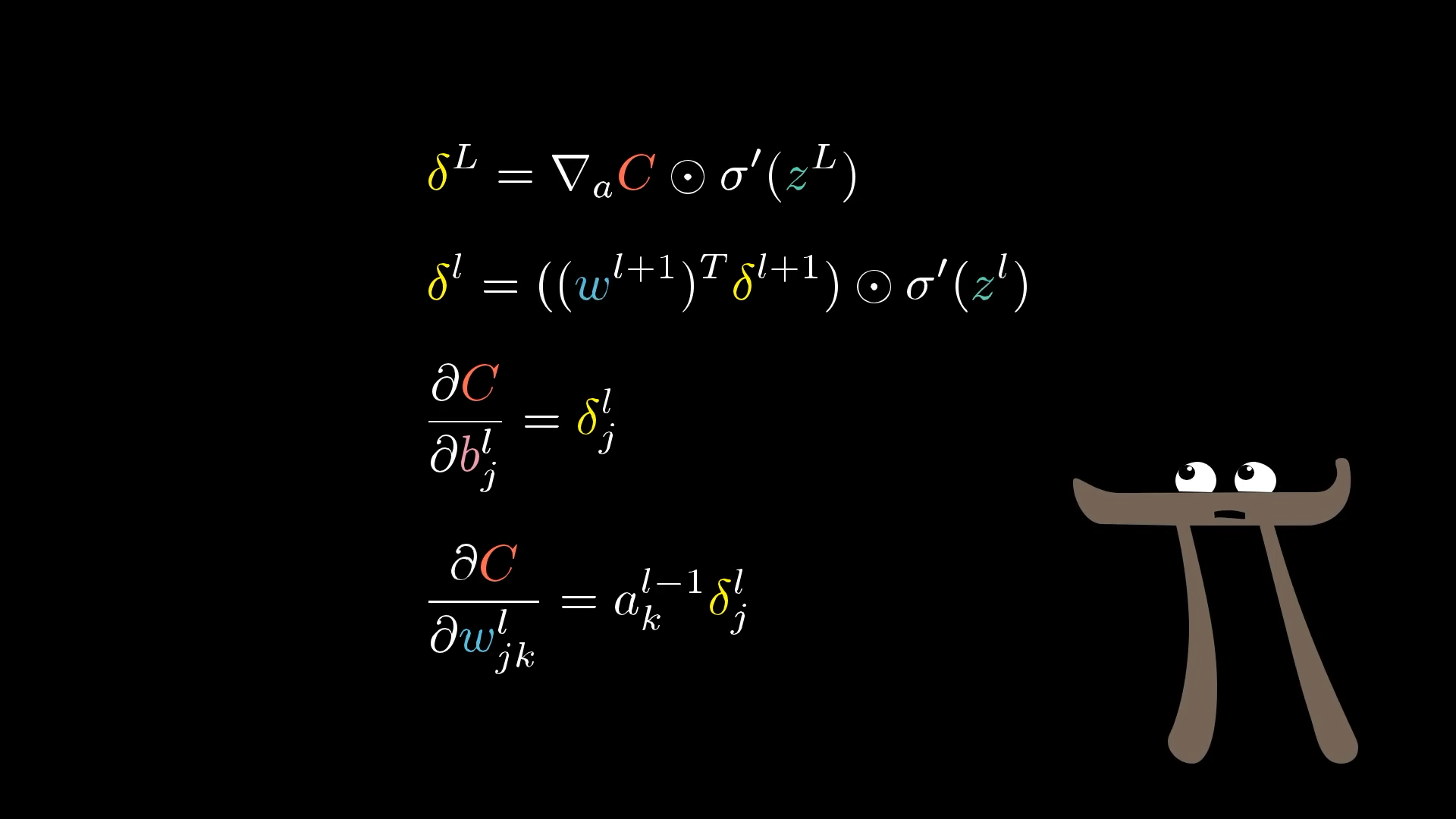
Remember, the negative gradient of the cost function is a 13,002-dimensional vector that tells us how to nudge all the weights and biases to decrease the cost most efficiently. Backpropagation, the topic of this lesson, is an algorithm for computing that negative gradient.
Thinking about the gradient vector as a direction in a 13,002-dimensional space is, to put it lightly, beyond the scope of our imaginations.

Direction in 13,002 dimensions?!?
So as we talked about in the previous lesson, it's helpful to consider it this way: The magnitude of each component of the gradient tells you how sensitive the cost function is to each corresponding weight and bias.
For example, let’s say you compute the negative gradient, using the process I’m about to describe, and the component associated with the weight on one edge comes out to be 3.2, while the component associated with some other edge is 0.1:
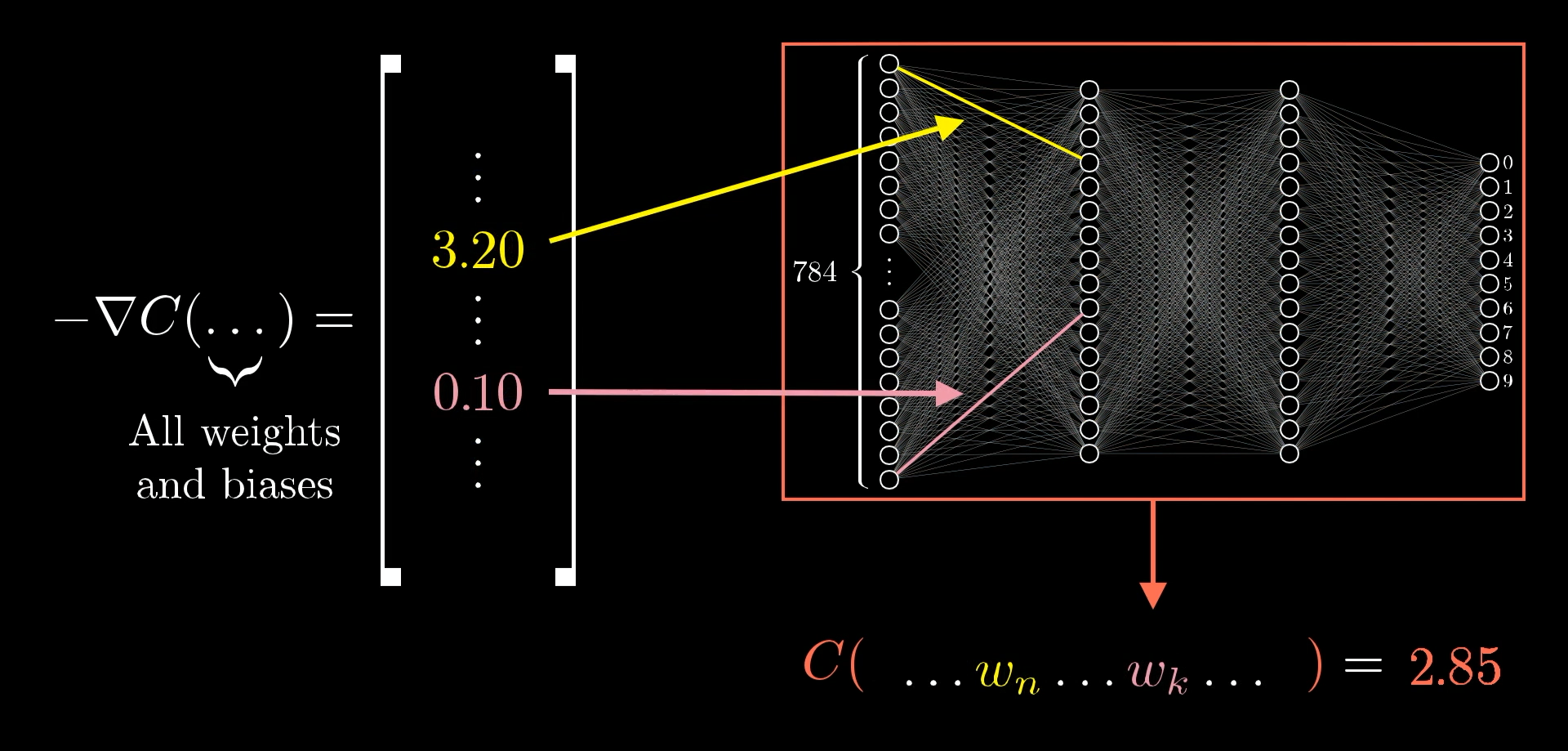
Suppose the entry of the gradient vector associated with one weight is 32x as large as the entry associated with some other weight.
The way to read this is that the cost function is 32 times more sensitive to changes to that first weight. So if you were to wiggle the value of that weight a bit, it’ll cause a change to the cost function 32 times greater than what the same wiggle to the second weight would cause.
Changing a weight that has a larger magnitude in the negative gradient vector has a bigger effect on the cost.
The Intuition for Backpropagation
When I first learned backpropagation, the most confusing aspect was just the notation and index chasing of it all.
There’s a lot of notation here. What does it all mean!?
For this article, let’s begin with a complete disregard for notation and instead step through the effect that each training example has on the weights and biases. Hopefully, these effects will feel intuitive so that by the time we return to the notation, it acts to articulate something you already know, rather than acting as a code to be decrypted.
Because the full cost function involves averaging a certain cost-per-example for all the tens of thousands of training examples, the way we adjust all the weights and biases for a single gradient descent step also depends on every single example. Or, rather, in principle it should, but for computational efficiency, we’ll do a little trick later to keep you from needing to hit every single example for every single step.
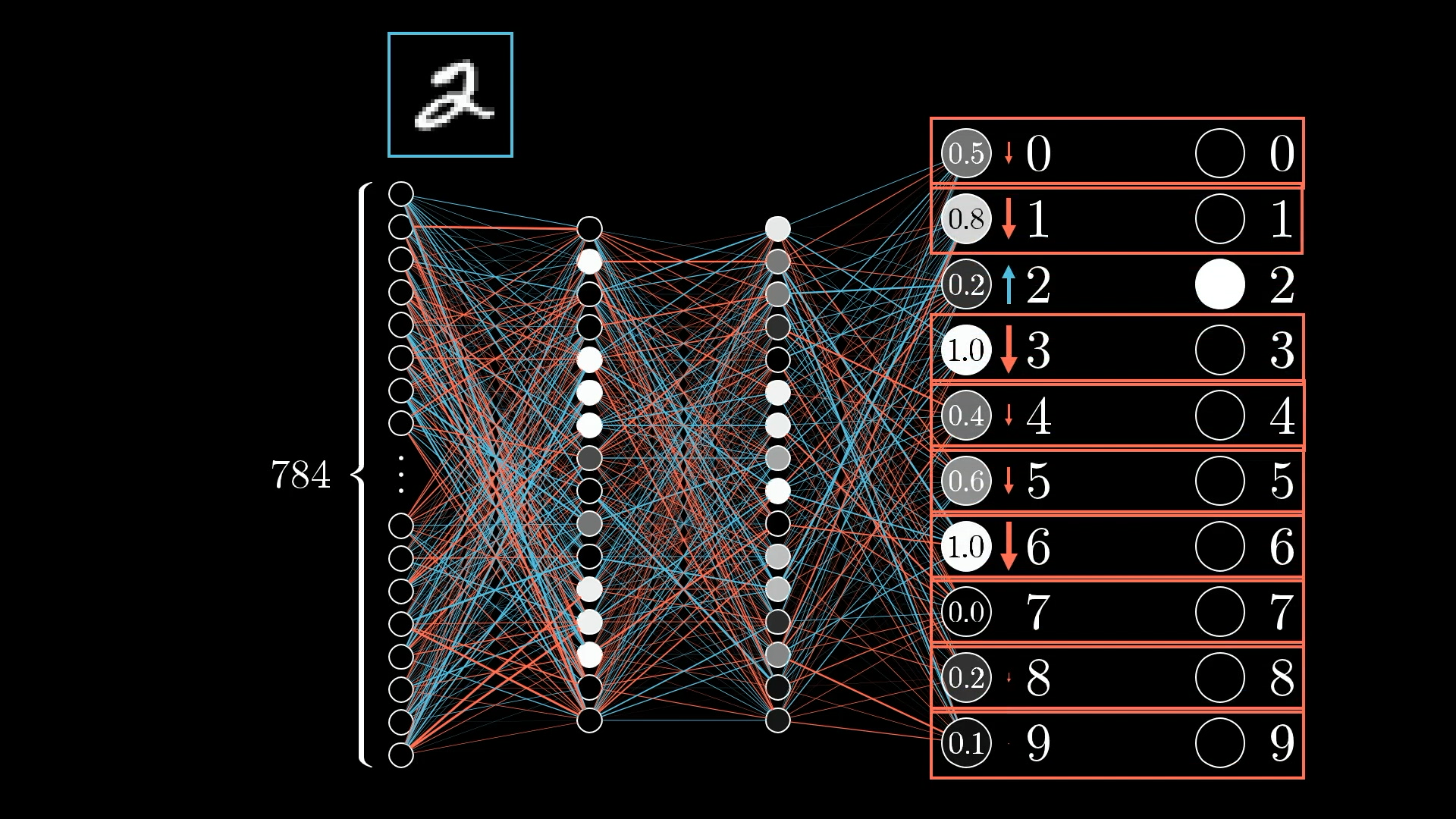
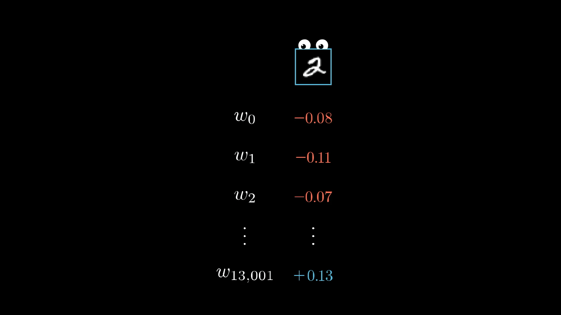
Right now, though, focus your attention on a single example, this image of a 2:
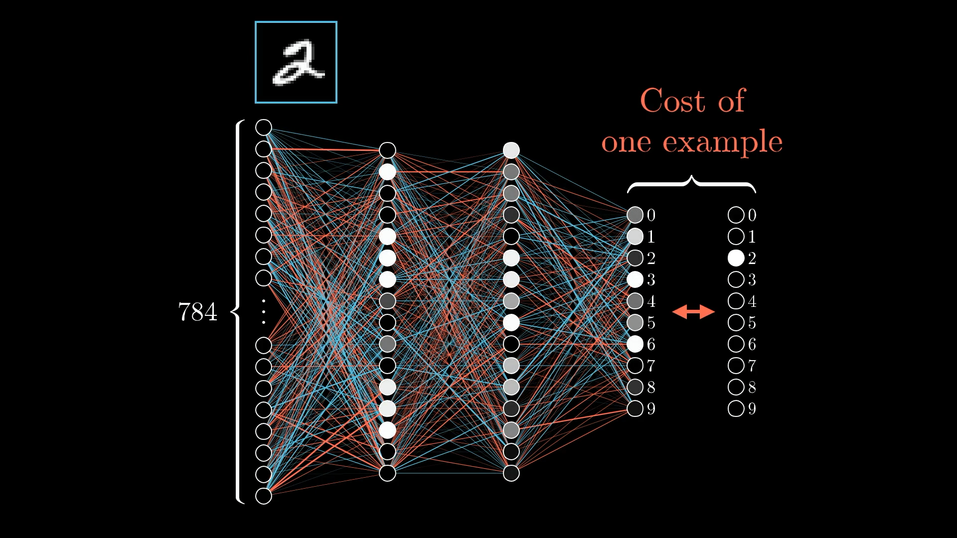
How can we adjust the weights and biases to improve the network’s performance on this image?
What effect does this one training example have on how the weights and biases should be adjusted?
Because the network is not yet well trained, the activations in that output layer are effectively random. That's no good; we want to change these activations so that they properly identify the digit 2.
But remember, we only have control over the weights and biases of the network. So we will have to nudge those weights and biases in a way that improves the output.
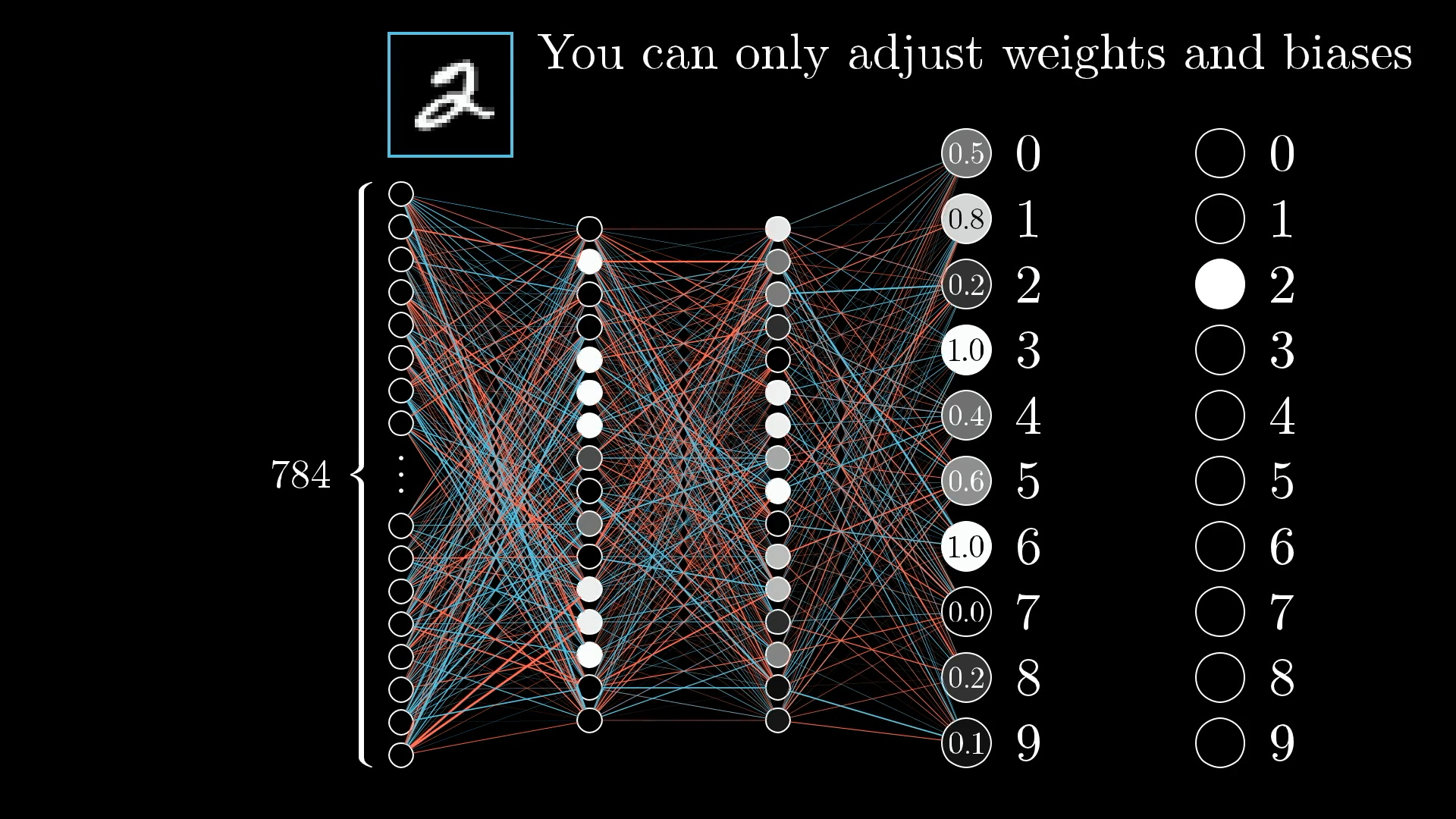
The activations in the output layer are trash, and we need to fix them by adjusting the weights and biases.
Although we can't directly change the activations, it’s helpful to keep track of what adjustments we wish to take place in this output layer.
Since we want the network to classify this as a 2, we want the digit 2 neuron’s value to be nudged up while all the others get nudged down:
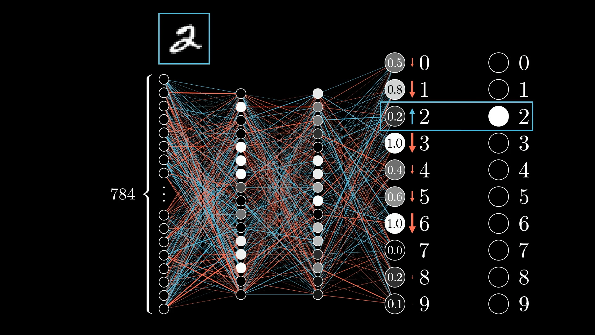
Moreover, the sizes of these nudges should be proportional to how far off each output value is from the target. Neurons that are way off require big nudges, but neurons that are pretty close to correct only require little nudges.
Zooming in further, let’s focus on the one neuron whose activation we wish to increase:
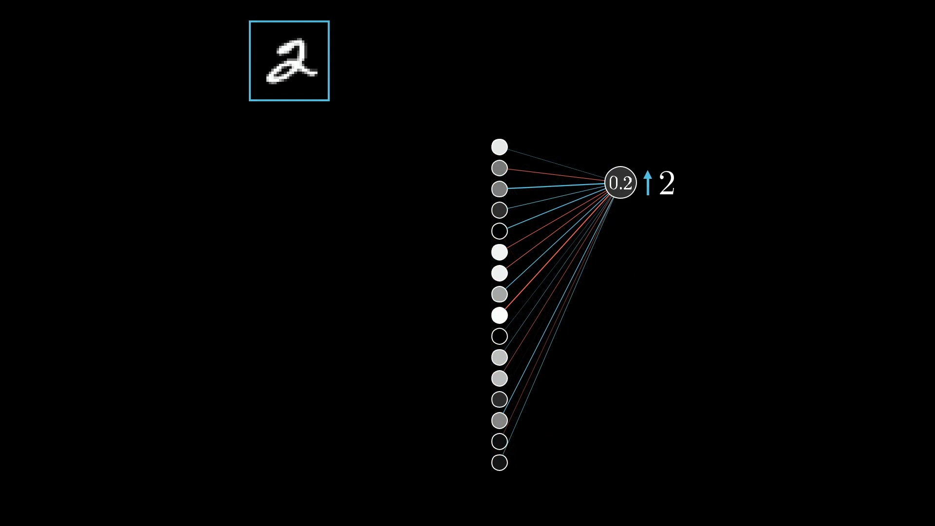
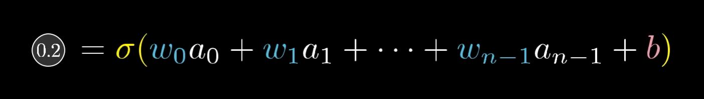
Remember that its activation value (in this case 0.2) is defined as a weighted sum of all activations from the previous layer, plus a bias, which is then plugged into something like the sigmoid squishification or a ReLU:
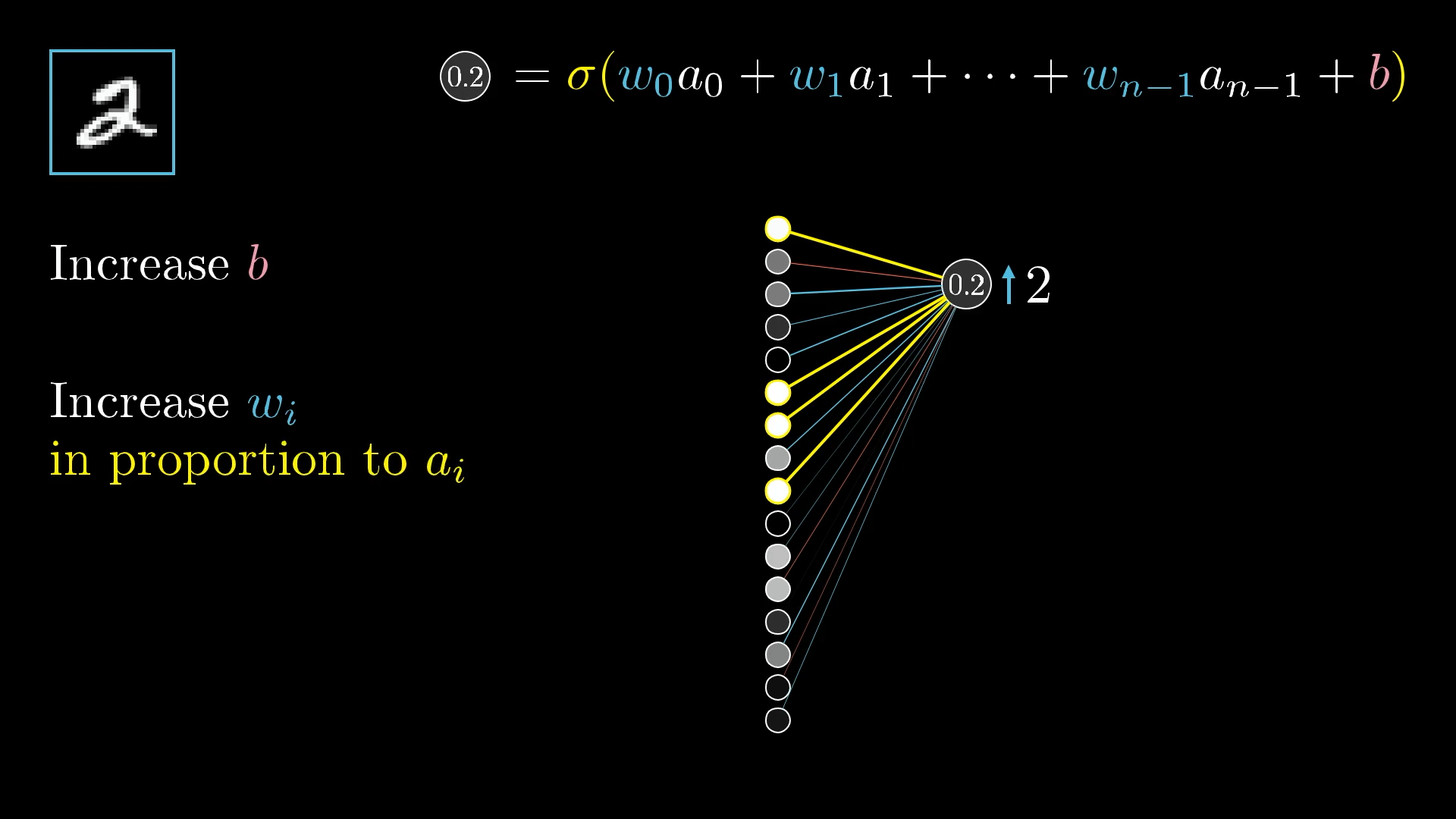
So there are three avenues that can team up together to increase this activation:
- Increase the bias
- Increase the weights
- Change the activations from the previous layer
Changing the Bias
Changing the bias associated with a neuron is the simplest way to change its activation. Unlike changing the weights or the activations from the previous layer, the effect of a change to the bias on the weighted sum is constant and predictable.
Since we want to increase the activation of the digit-2 output neuron we've been discussing, how should its associated bias be adjusted? What about the biases associated with all the other output neurons for this training example?
Changing the Weights
How should the weights be adjusted? Notice, because they are being multiplied by the activations, the weights have differing levels of influence:
Changing the weights associated with large activation values will have a stronger effect than changing the weights associated with small activation values.
The connections with the brightest neurons from the preceding layer have the biggest effect since those weights are multiplied by larger activation values. So increasing one of those weights has a bigger influence on the cost function than increasing the weight of a connection with a dimmer neuron. (Again, this is all only insofar as this one training example is concerned.)
Remember, when we talk about gradient descent, we don’t just care about whether each component should be nudged up or down. We care about which ones give you the most bang for your buck.
To get the most bang for your buck, adjust the weights in proportion to their associated activations.
This, by the way, is at least somewhat reminiscent of a theory in neuroscience for how biological networks of neurons learn, Hebbian theory, often summed up in the phrase “neurons that fire together wire together.” Here, the biggest increases in weights—the biggest strengthening of connections—happens between neurons that are the most active and the ones which we wish to become more active.
In some sense, the neurons that fire while seeing a 2 get more strongly linked to those firing while thinking about a 2.
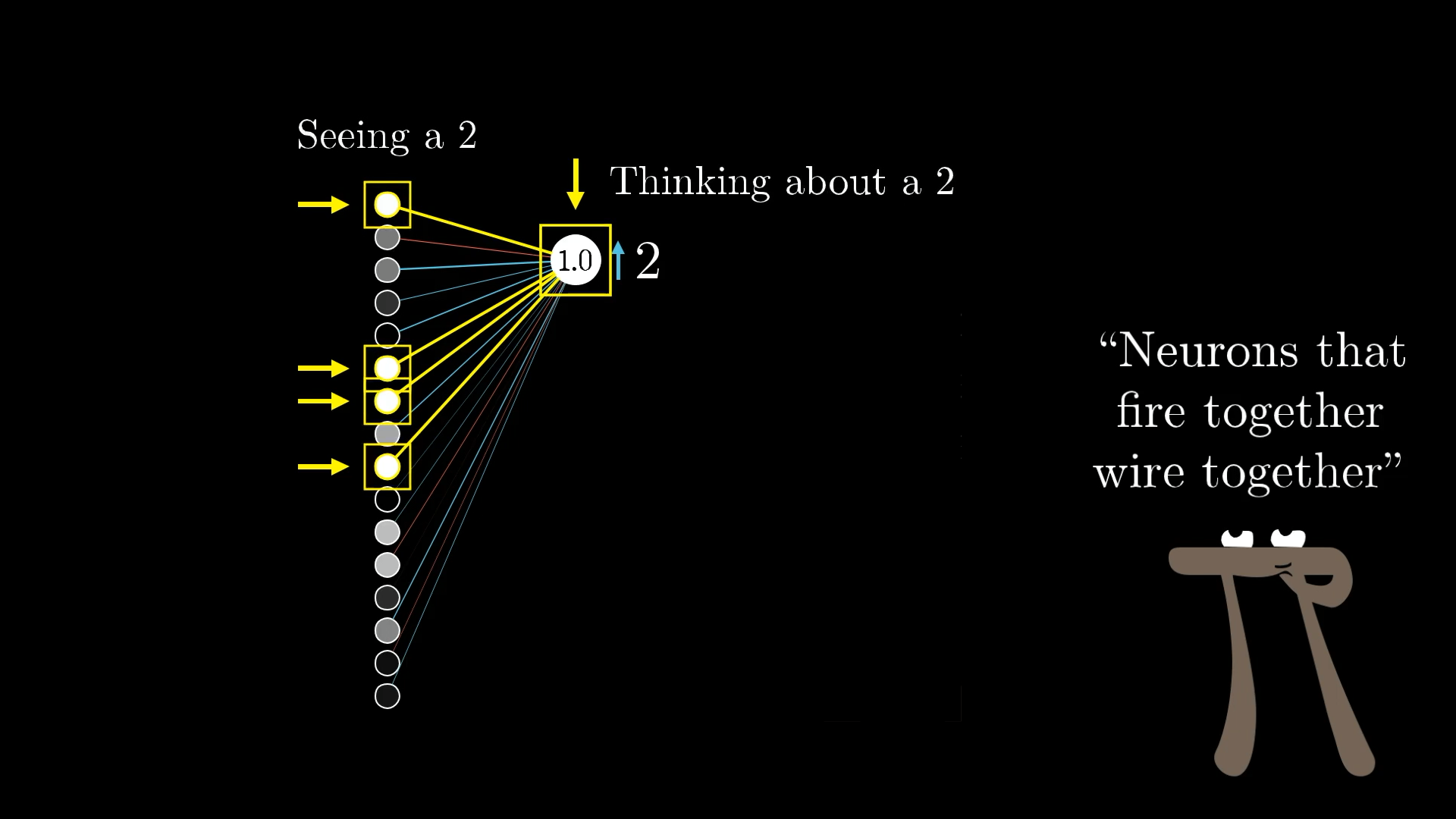
Connections are strengthened between neurons that should be activated at the same time.
The analogy is not perfect since the untrained network is not really “thinking” about a 2 when it sees this example; it’s more that the label on the training data is hardcoding what the network should be thinking about. Still, it’s satisfying to know that buried beneath all the calculus and linear algebra typically used to describe backpropagation, the actual changes happening to the weights with each training example mirror the ideas of Hebbian theory.
Changing the Activations
The third way we can help increase this neuron’s activation is by changing all the activations in the previous layer. Namely, if everything connected to that digit-2 neuron with a positive weight was brighter, and if everything connected with a negative weight was dimmer, that digit-2 neuron would be more active.
Similar to the weight changes, you’ll get the most bang for your buck by seeking changes proportional to the size of the corresponding weights:
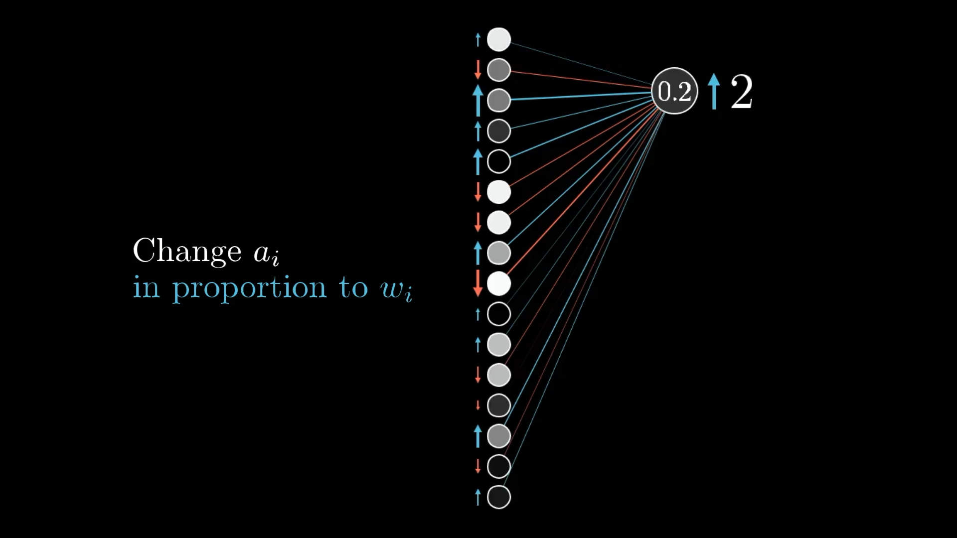
Just like changing weights in proportion to activations, you get the most bang for your buck by increasing activations in proportion to their associated weights.
Of course, we cannot directly influence these activations. We only have control over the weights and biases. But just as with the last layer, it’s helpful to keep note of the desired changes.
We can’t influence the activations in the previous layer directly. But we can change the weights and biases that determine their values!
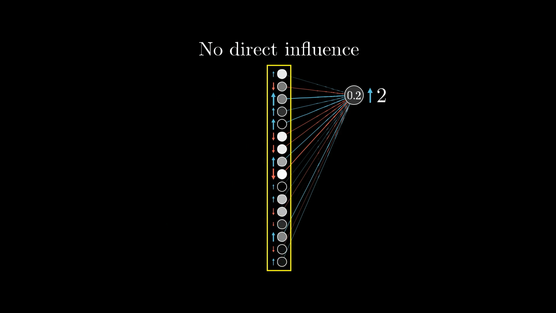
Remember, this is only what that one digit-2 output neuron wants. We also want all the other neurons in the last layer to become less active, and each of those other output neurons has its own influence on what should happen to the second-to-last layer.
We want to adjust all these other output neurons too, which means we will have many competing requests for changes to activations in the previous layer.
So the desire of this digit-2 neuron is added together with the desires of all the other nine neurons. Each has its own suggested nudge for that second-to-last layer, again in proportion to the corresponding weights and in proportion to how much each neuron needs to change.
It’s impossible to perfectly satisfy all these competing desires for activations in the second layer. The best we can do is add up all the desired nudges to find the overall desired change.
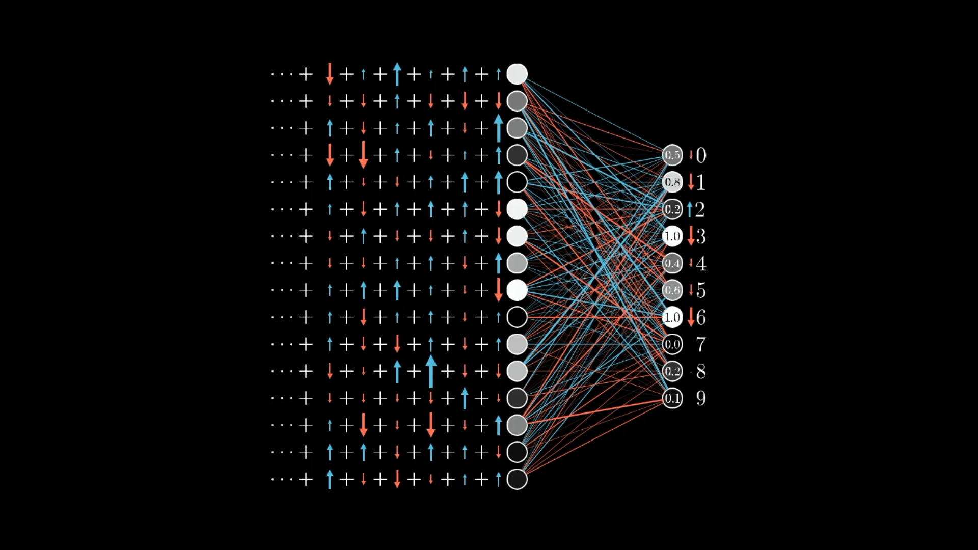
Here is where the idea of propagating backward comes in. By adding all these desired effects, you can get a list of the nudges you want to happen to this second-to-last layer. From there, you can recursively apply the same process to the relevant weights and biases determining those values, repeating this process as you move backward through the network.
Repeating for All Training Examples
Everything we just stepped through only records how a single training example wishes to nudge each of the many, many weights and biases.
So far we’ve only identified the nudges to the weights and biases that would improve our results for this digit 2. But we also need to account for all the other digits!
If we only listened to what that image of a 2 wanted, the network would ultimately be incentivized to just classify all images as a 2.
To zoom out a bit, you also go through this same backpropagation routine for every other training example, recording how each of them would like to change the weights and biases. Then you average together all those desired changes.
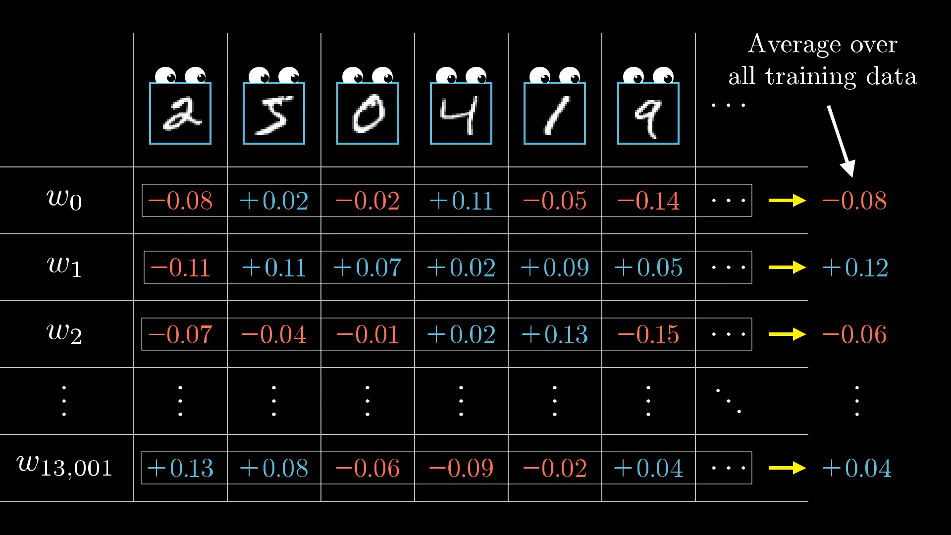
Each training example has its own desire for how the weights and biases should be adjusted, and with what relative strengths. By averaging together the desires of all training examples, we get the final result for how a given weight or bias should be changed in a single gradient descent step.
The collection of these averaged nudges to each weight and bias is, loosely speaking, the negative gradient of the cost function! Or at least something proportional to it.
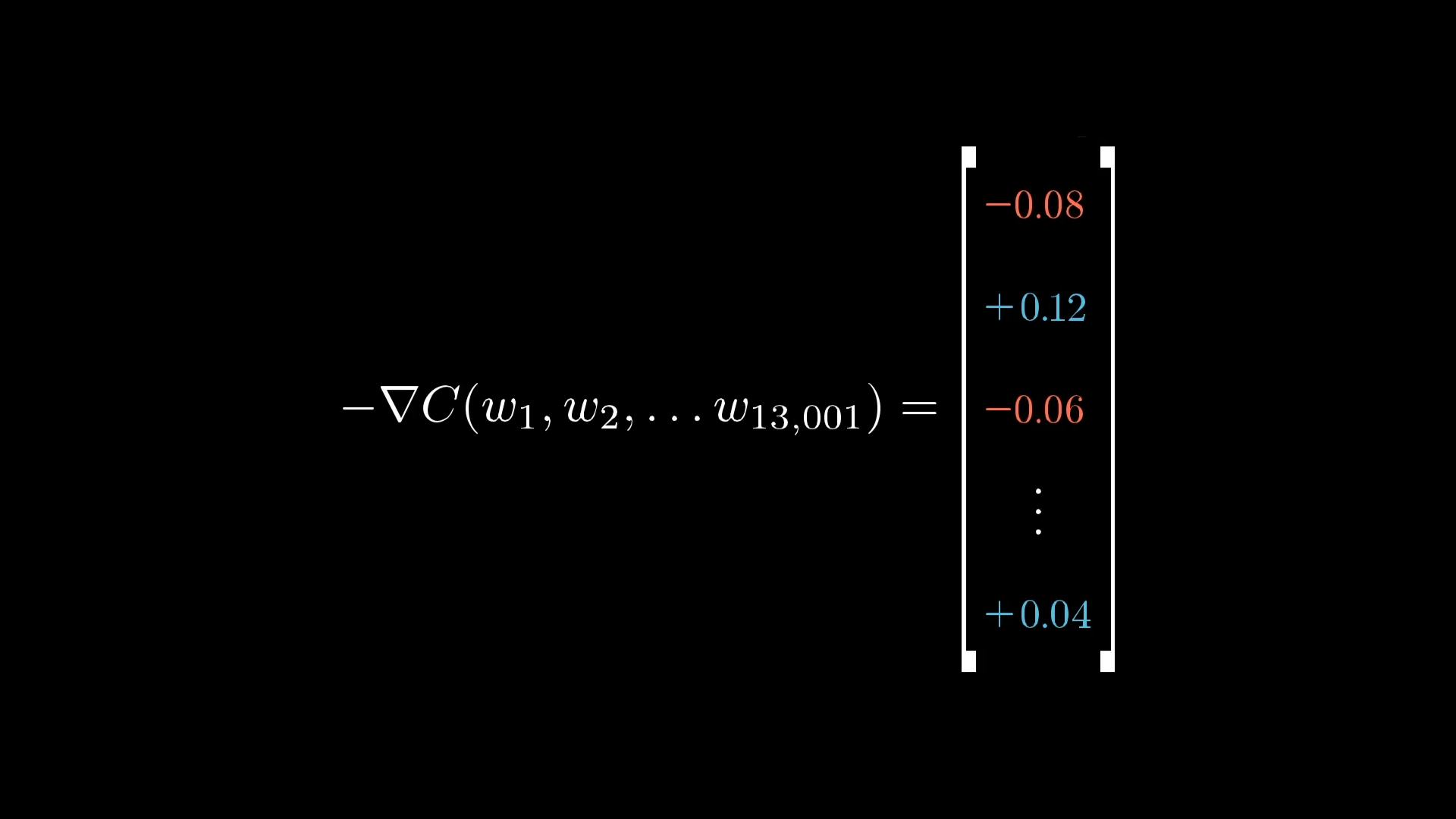
The result of all this backpropagation is that we’ve found (something proportional to) the negative gradient!
I say “loosely speaking” only because I have yet to get quantitatively precise about these nudges. But if you understood each change I referenced above, why some are proportionally bigger than others, and how they all need to be added together, then you understand the mechanics for what backpropagation is actually doing.
Stochastic Gradient Descent
In practice, it takes computers an extremely long time to add up the influences of every single training example for every single gradient descent step. Instead, there’s a clever trick for speeding up the process in a way that involves more total gradient descent steps but much less time for each one.
Randomly shuffle your training data and divide it into a bunch of mini-batches, having, say, 100 training examples each.
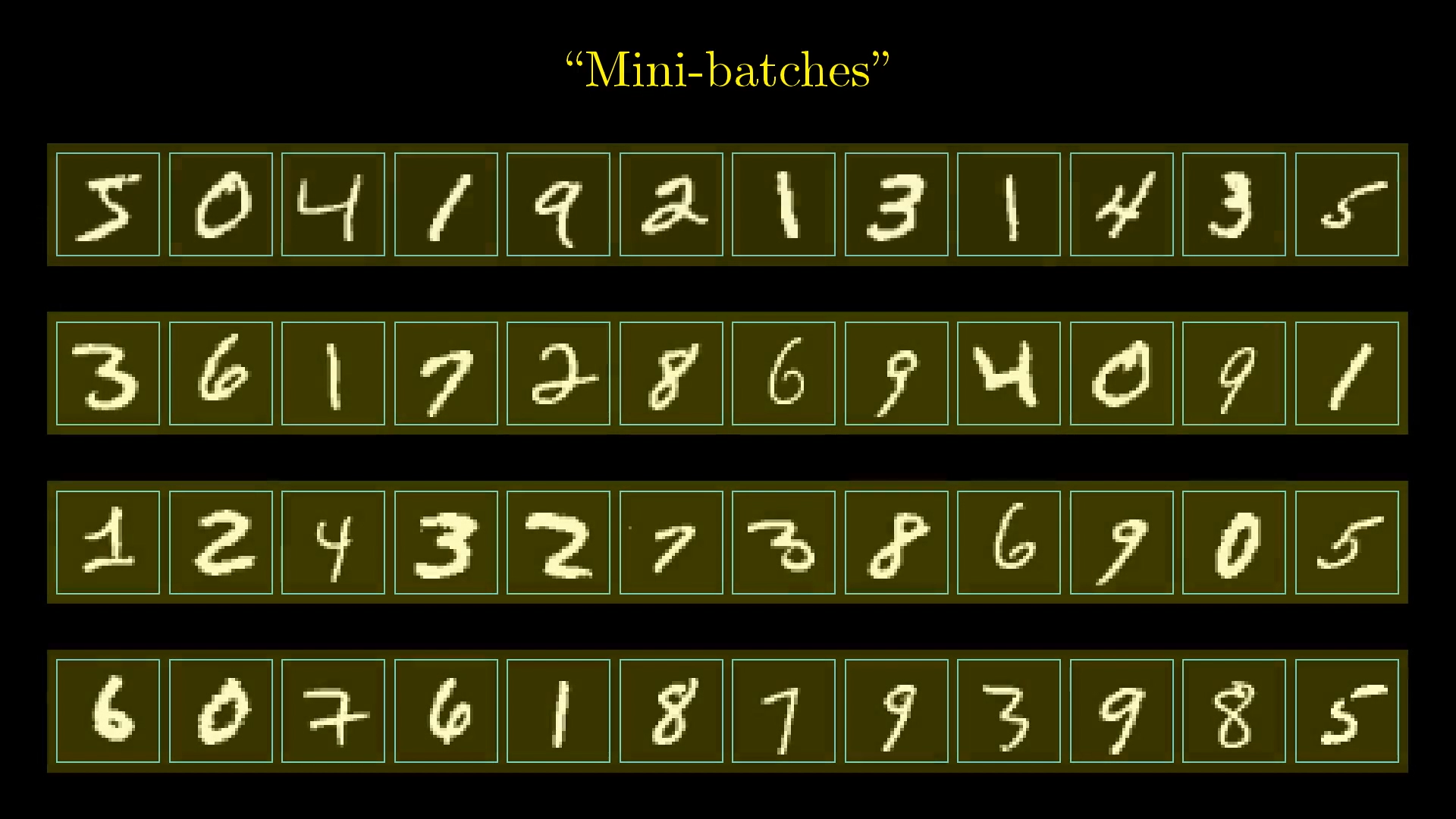
Then you compute a gradient descent step according to each minibatch rather than the entire set of training examples. It won’t give you the actual gradient of the cost function, which depends on all the training data, so it’s not the most efficient step downhill. But each mini-batch gives a pretty good approximation, and if there are 100 minibatches, each step takes 1/100th of the total time. And after 100 steps, each piece of training data will have had its chance to influence the final result.
With these mini-batches, which only approximate the gradient, the process of gradient descent looks more like a drunk man stumbling aimlessly down a hill but taking quick steps rather than a carefully calculating man who takes slow, deliberate steps downhill.
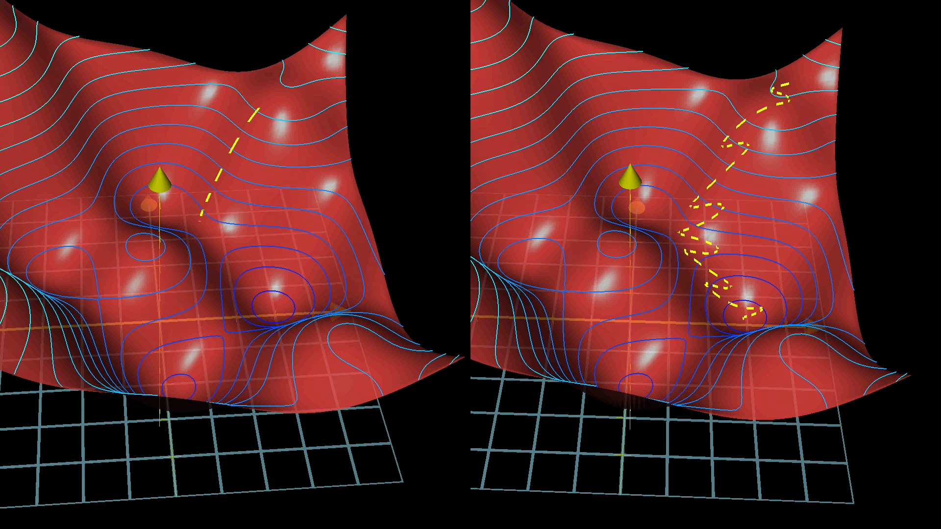
Using mini-batches means our steps downhill aren’t quite as accurate, but they’re much faster.
This is referred to as Stochastic gradient descent.
Conclusion
With that, every line of code that would go into implementing backpropagation corresponds to something you have now seen, at least in informal terms. But sometimes, knowing what the math does is only half the battle, and just representing the damn thing is where it gets all muddled and confusing.
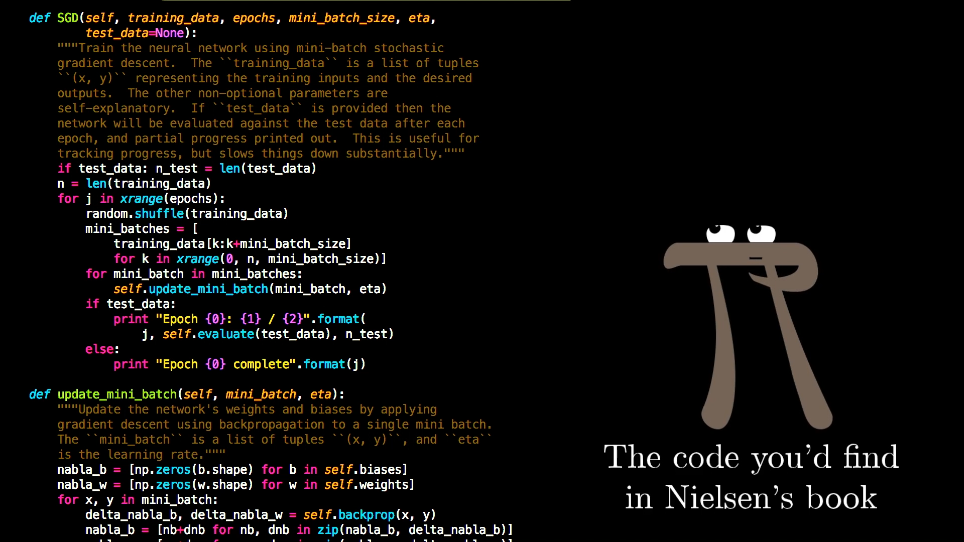
You have now seen the intuition behind all the code (like you might find in Nielsen’s book) that goes into building a simple neural network.
So for those of you who want to go deeper, the next lesson goes through the same ideas presented here, but in terms of the underlying calculus, which should hopefully make it more familiar as you see the topic in other resources.
Thanks
Special thanks to those below for supporting the original video behind this post, and to current patrons for funding ongoing projects. If you find these lessons valuable, consider joining.